Google Sheets

Fun with Google Sheets, Part 4

I’m back today with more tips and tricks to make Google Sheets fun and amazing.

Filter by Color

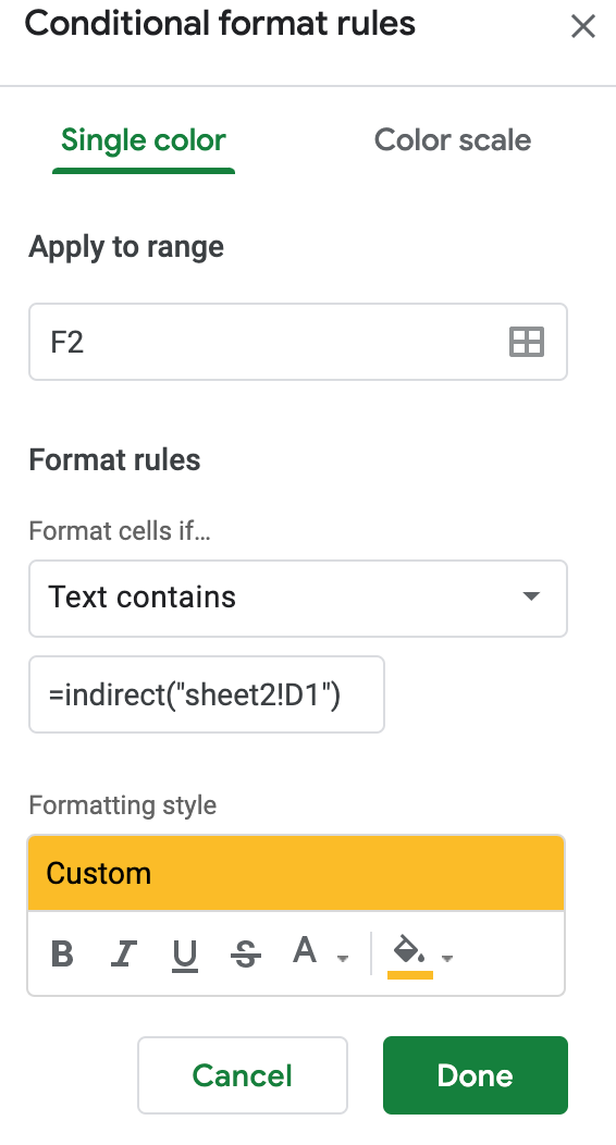
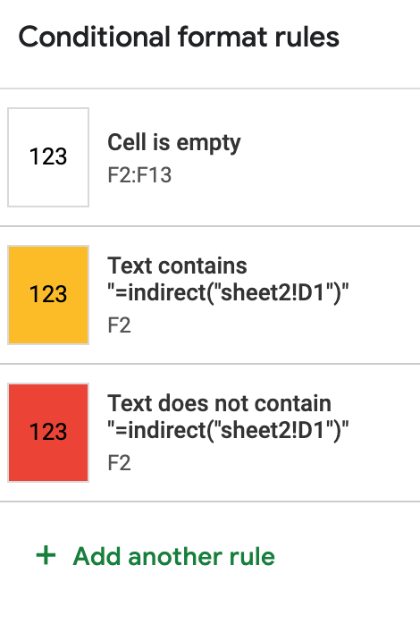
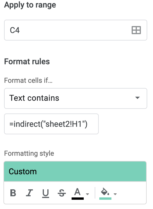
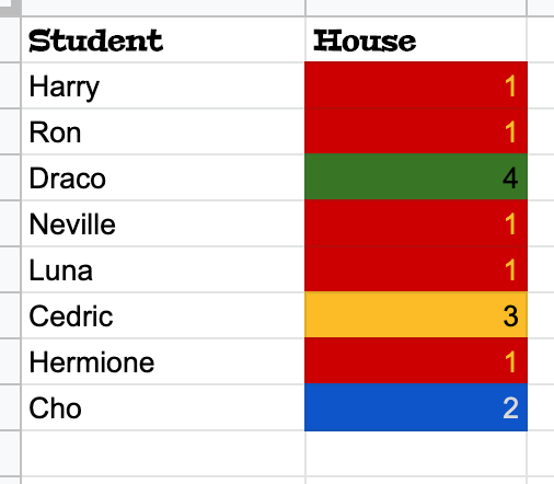
If you have set up your sheet to change colors using conditional formatting (Fun With Sheets 2), then you can filter by color to see entries that are a certain color.

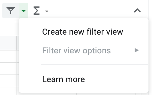
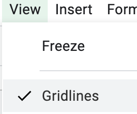
Highlight the cells you want to sort, then select the funnel looking tool on the right of the toolbar. Select Create new filter view.

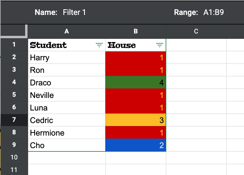
The view changes and these little upside down triangles show up on the first line.

I’m going to click the triangle on House to filter.

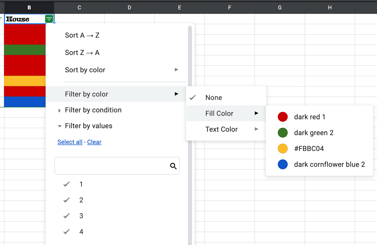
I selected dark red 1 to get my Gryffindor students.

*Note that you can also filter by text color if you prefer colored text instead of colored cells.

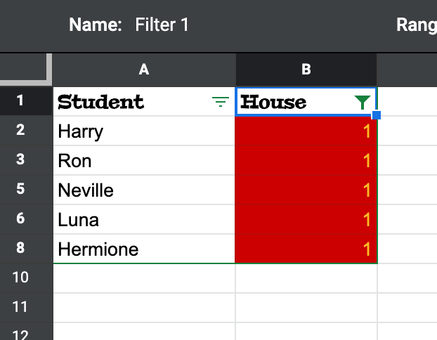
A now I have just my Gryffindor students.

Hiding Cells/Sheet

If you’ve been following along with the Google Sheets activities I’ve been creating, then you may already know these tricks. I use them in my activities all the time.

Hiding Cells

Sometimes you don’t want part of your cells to show. Maybe you have some calculations happening, maybe some answers. You can hide those sheets so students can’t see them. Now, a tech savvy student might notice, but we will get to that in the next step.

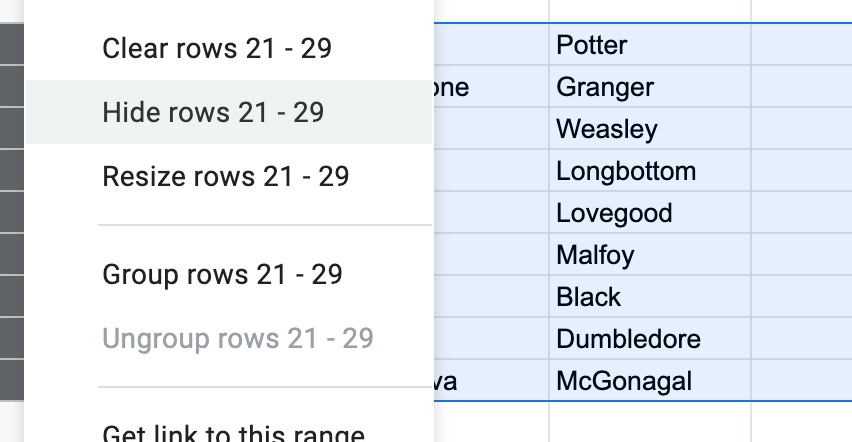
Highlight the rows you want to hide (works for columns too), right click and select hide rows.

Once the rows (or columns) are hidden, you can see the arrows indicating there are hidden cells.

Hide Sheet

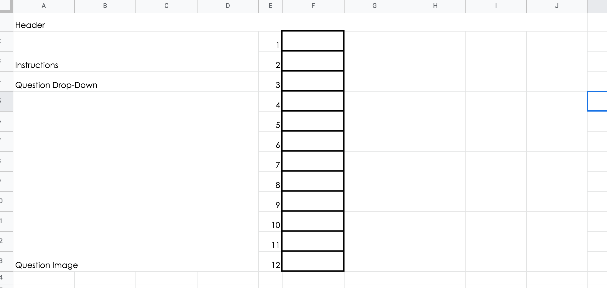
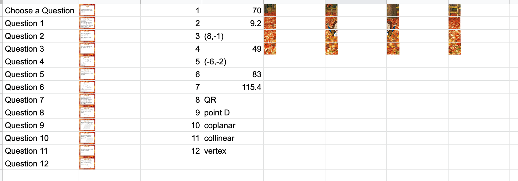
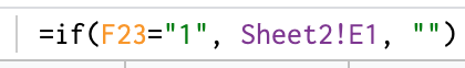
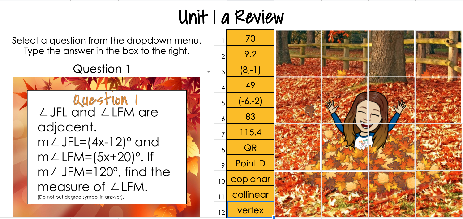
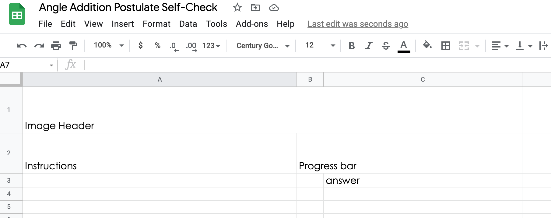
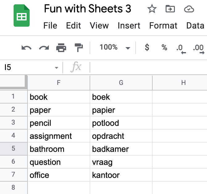
You can also hide an entire sheet from view. If you create an activity and put the images and answers on Sheet 2, you don’t want students to be able to see that.

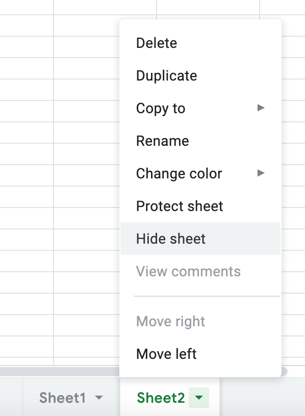
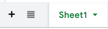
Once the sheet is ready, right click and hide sheet.

Protect Cells/Sheets

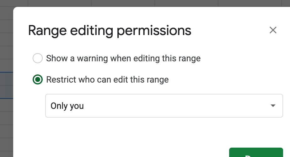
Once you have hidden your cells and sheets, you want to prevent tech savvy students from unhiding them. You can protect these so you are the only person with access.

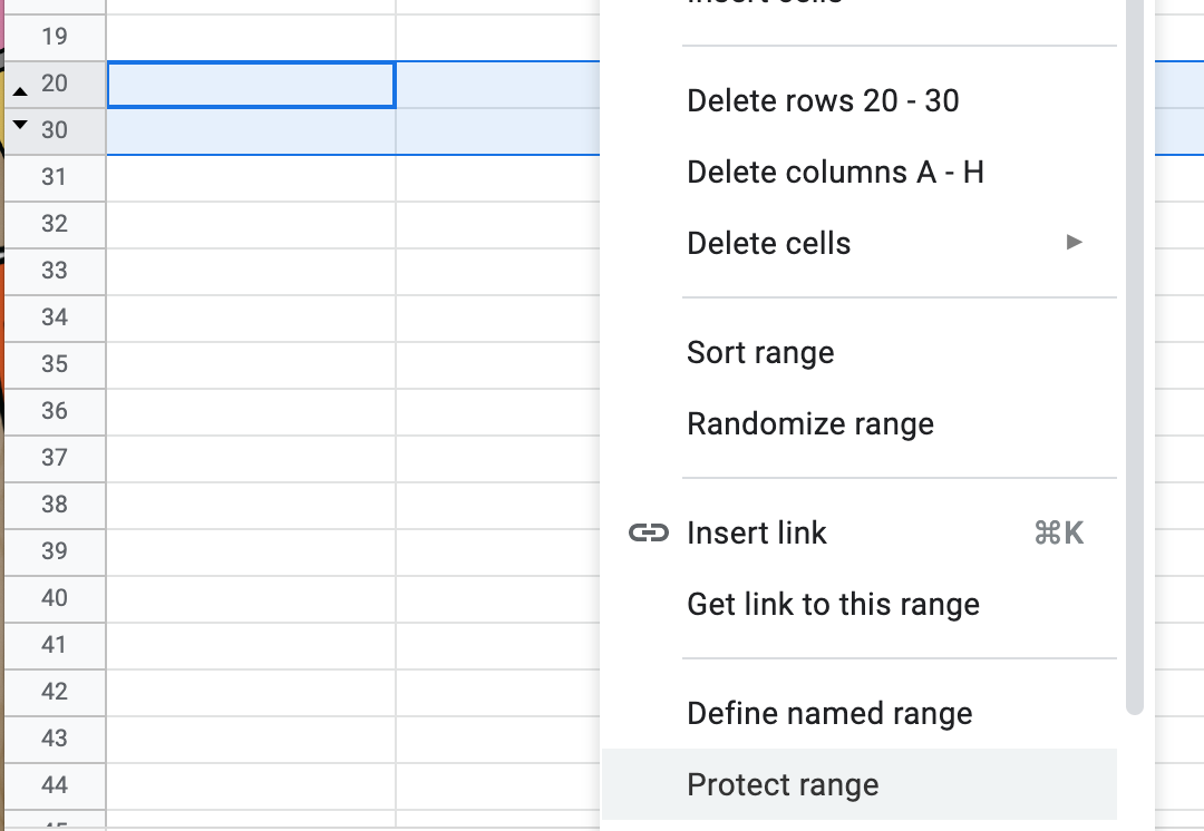
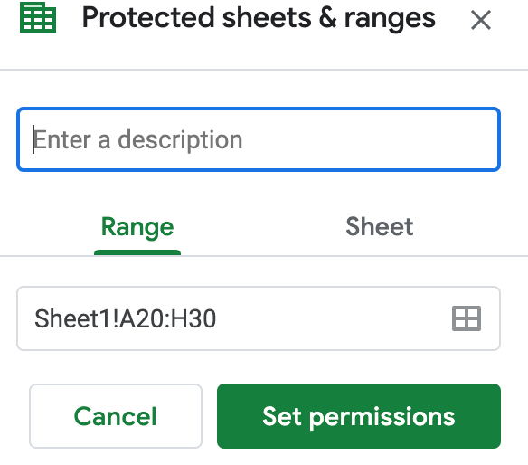
Highlight the cells you want to protect, right click, and select protect range.

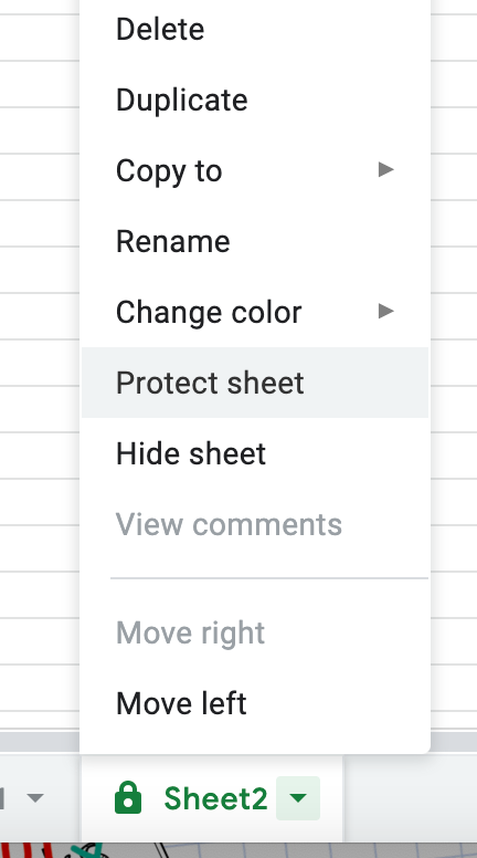
You can do the same thing with the sheet, by right clicking on the sheet and setting protection.

The only caveat with this is once a student makes a copy, like they have to do when they solve a puzzle, the YOU in “only you can make a change” is THEM. So they can now see your Sheet 2 and hidden cells if they know how to unhide. For this reason, I like to make my font color white so it disappears and I place the answers where they have to scroll a lot to find them. Is it perfect? No. But these activities are fun and work well for digital escape rooms or review so I will continue to make them.

I hope this series is helping you embrace the amazingness that is Google Sheets!

See previous Fund with Google Sheets posts:

Digital Escape Rooms, formative assessment, Geometry, Google Sheets, Self-Checking

Self-Checking Magic Squares Sheet

This tutorial is combining two ideas together that I have previously shared. This first is a Magic Squares sheet by Jason Pullano, and the other was a recent post about self-checking sheet. This activity is great for a self-checking activity or as a clue in a digital escape room.

Many of the steps are the same, so I am just reposting them below so you don’t have to flip screens.

Create your Questions

I find it’s easier to have my questions and images (if needed) ready to go before I begin building the spreadsheet.

I’m using this for a Geometry review so I’ve created my images in advance in a Google Slide and I changed the page size to the standard 4:3. I can download each card as a PNG or JPG image to use in my self-checking activity.

Create the image

This activity loads an image into squares one at a time as a correct answer is entered. You will need to decide how many squares you want. I went with a 4×4 grid.

I used Google Drawing. In page set-up I set the size to 10 x 10.

Once your image is designed, place a table on top of it and drag it to fill the screen. I learned this trick from Jason Pullano. The table creates a perfect grid and you don’t have to worry about placement of the lines.

Now you crop your image. There is more than one way to do this but I chose to use my snipping tool and just snip each section. I found it helpful to zoom in to get a good snip.

Open Sheets

Now we will put this all together.

I start with my blocks of information. I merged cells to create the sections for instructions, question images, and also to create my grid. By selecting columns G-J and right clicking, I can resize my columns to 99. Do the same for rows 2-3 and resize to 33. This should give us squares.

I just typed in my header this time, but you could always create a colorful header like we did the last time. If you create the header image, insert instructions are below.

Place images and answer in a new tab.

Click the plus button in the bottom left corner of your spreadsheet. This will create a new tab in Sheets. This will be the location for out images and answers.

Place the images (insert image) for the questions and for the square reveal. They can be VERY TINY. It’s ok. It will scale to fit the size we allow it.

We also want to place the answers to our questions here. We are going to hide the tab later so students don’t see it.

Dropdown menu

Start with the dropdown menu where you have the word instructions. Place the same words, Choose a Question, Question 1, etc. in your list. You can view a tutorial here.

Now right below that, you will enter a vlookup code.

=vlookup(A4,Sheet2!A1:B13,2,0)

This is telling sheets to see what word is selected in A4 (Choose a question, Question 1, etc., then go to sheet 2 and select the image that matches my words that are in column A starting at A1 and my images are in column B ending at B13.

Answers

Now let’s set the conditional formatting for our answers. There is a tutorial for conditional formatting in the link above as well.

I’m going to have three rules for each cell. If the cell is empty, I want it to be transparent. If the cell has an entry it will be gold for correct or red for incorrect.

It’s a little tricky to get conditional formatting from another sheet.

Here is what you would type in:

We will do the same thing to get a wrong answer but select text does not contain and type in the same formula and change the color to red.

Repeat for the remaining answers.

*This seems like a lot of work, but this process allows you to use this template again simply by changing the images and answers in Sheet 2.

Load Image

Now we need to load an image square. When an answer is correct, we want a square to load in an image space.

Below the fun stuff in Sheet 1, I have the sheet respond with 1 if an answer is correct and 0 if it’s incorrect using the following formula:

Once you return, there will be a little blue box in bottom right corner. You can drag that box down 10 spaces and it will auto fill the formula for you.

Choose a square you want to load. For this example, if the answer is correct it will go to sheet 2 and load the image in D1. You just need to make sure you load them in random order and that you include each one.

I have 16 boxes and only 12 questions so a few of my questions load to squares.


Clean it up and Assign

I like to hide the parts of the sheet we don’t need.

I’m going to highlight columns K-Z and right click and hide those cells

You can also hide the rows that have your adding trick on them by doing the same thing.

I’m also going to hide the sheet with my answers on it. Now a spreadsheet savvy student will now how to unhide this so you can always password protect the sheet so they can’t access it.

Don’t forget to set it to make a copy for every student in your LMS.

Here is the final result with all of the answers filled in:

These are so much fun. You can even get more advanced and have one image load and it changes to another image as you get the answer correct.

You can always just use the created spreadsheet below as a template if you don’t want to make your own. Just switch out the images and answers on Sheet 2.

If you make one, please let me know. I love to make these and my students love to complete these.

differentiation, Geometry, Google Sheets

Self-Checking Google Sheets

This is not the first self-checking Google Sheet tutorial I’ve shared. This is just ANOTHER example of what you can do with Google Sheets. You can see the Pixel Art tutorial here. I’ve learned a few new tricks since then and have improved the process making it harder for students to find the answers in the code. It’s still possible, just more difficult.

Create your Questions

I find it’s easier to have my questions and images (if needed) ready to go before I begin building the spreadsheet.

I’m using this for Angle Addition Postulate so I’ve created my images in advance in a Google Slide and I changed the page size to the standard 4:3. I can download each card as a PNG or JPG image to use in my self-checking activity.

Progress Bar

For this type of self-checking activity you can have a progress bar or progress circle to tell students how many they have correct. Or you can just have the number of correct answers in the corner. For this tutorial, I’m going to use the progress bar

I drew my own, just for fun, but you could create these in Google Drawing or Google Slides. You will need one image for each increase in the bar or circle.

Open Sheets

Now we will put this all together.

I start with my blocks of information.

I created my header in Google Drawing. I will insert the image in the cell.

Place images and answer in a new tab.

Click the plus button in the bottom left corner of your spreadsheet. This will create a new tab in Sheets. This will be the location for out images and answers.

Place the images (insert image) for the questions and for the progress bar. They can be VERY TINY. It’s ok. It will scale to fit the size we allow it.

We also want to place the answers to our questions here. We are going to hide the tab later so students don’t see it.

Dropdown menu

Start with the dropdown menu where you have the word instructions. Place the same words, Choose a Question, Question 1, etc. in your list. You can view a tutorial here.

Now right below that, you will enter a vlookup code.

=vlookup(A3,Sheet2!D1:E12,2,0)

This is telling sheets to see what word is selected in A2 (Choose a question, Question 1, etc., then go to sheet 2 and select the image that matches my words that are in column D starting at D1 and my images are in column E ending at E12.

Answers

Now let’s set the conditional formatting for our answers. There is a tutorial for conditional formatting in the link above as well.

I’m going to have three rules for each cell. If the cell is empty, I want it to be transparent. If the cell has an entry it will be green for correct or yellow for incorrect.

It’s a little tricky to get conditional formatting from another sheet.

Here is what you would type in:

We will do the same thing to get a wrong answer but select text does not contain and type in the same formula and change the color to yellow.

Repeat for the remaining answers.

*This seems like a lot of work, but this process allows you to use this template again simply by changing the images and answers in Sheet 2.

Progress Bar

Now we need to add the progress bar. When an answer turns green, we want the progress bar to advance. Basically, you are adding the amount of correct answers together and telling the progress bar to load an image based on the number of correct answers.

I have the number of correct answers add somewhere hidden on sheet 1 (below or to the right of the current content) using the following formula:

Once you return, there will be a little blue box in bottom right corner. You can drag that box down 10 spaces and it will auto fill the formula for you.

Now we will add the columns. We will use this sum to load the correct images. I will hide these rows (or columns) later so students don’t see it.

Usually the =sum feature will work but for some reason it didn’t, so I just added each cell.

In the cell where the progress bar goes, we are going to use that same vlookup that we used earlier to load the correct image:


Clean it up and Assign

I like to hide the parts of the sheet we don’t need.

I’m going to highlight D=Z and right click and hide those cells

You can also hide the rows that have your adding trick on them by doing the same thing.

I’m also going to hide the sheet with my answers on it. Now a spreadsheet savvy student will now how to unhide this so you can always password protect the sheet so they can’t access it.

Don’t forget to set it to make a copy for every student in your LMS.

Whew! That was a lot of work! Here is your final product. You also now have a template to use if you want to create future projects. You can change out the progress bar, the questions, and the answers in Sheet 2. Yay!

I hope you find use for this tutorial. I know you can buy other templates like this on TPT, so if that’s how you roll, head on over to TPT. I personally like to create my own. It did take quite a bit of time, but now that the template is created, I can change it up with minimal effort.

And, because I’m nice, here is my completed activity if you want to use it as a template.

Spreadsheet

Slides with questions

Digital Escape Rooms, Distance Learning, formative assessment, Geometry, Google Sheets

Fun with Google Sheets – Part 3

It’s been a minute since we had a fun with Google Sheets so I decided to bring you another installment as school is starting or getting ready start for most of us.

Separate Names

I like to copy the names of my students from my gradebook screen or download an Excel file of students from our grade management system (we use PowerSchool). This copies first and last names but sometimes I just need first names. I DON’T want to go through a delete all of the names, especially since I usually have around 150 students.

Never fear, Google Sheets are here! You can EASILY separate the names into two columns.

Begin by typing the names into two columns, just as you want them to appear. It may take a few names, but once Google Sheets understands what you are doing, Smart Fill will pop up a suggestion. Click the checkmark and Sheets will do the rest.

You will do the same for the last name column. Then you have the entire sheet broken into first and last names. YAY! Such a time saver.

The process also works in reverse. So if you have first and last names in two columns, you can type both in the third column and smart fill will recognize the pattern and fill for you.

Google Translate

You can translate a list of words in Google Sheets. Type the list of words in one column. In the next column, type =googletranslate and and prompt will appear.

Next you want to click on the cell for the word you want to translate. Don’t worry, we don’t have to do this for every word, it will fill all of them in the end. It will place this cell into the formula, then put a comma and “auto” then a comma.

Now you need to find your two letter language code. These are called ISO codes and you can do a google search for them. Here is a link to the site I use. I’m translating to Dutch which is the code nl. So I will add the code in quotations and then close the parentheses.

One word is translated.

Now grab the blue box in the bottom right corner of that cell and drag down. You have translated all of the words.

Hiding Answers

I love to create interactive Google Slides for review games and escape room tasks. Most of the time the game works as it should. But every now and then a student figures out that you can click on the input box to see the answer. And, OF COURSE, they tell the rest of the class and now they are just entering the answer and not working out the problems.

Here is an example of a pixel art activity where this could be used. Many of mine have not been updated to this cell reference method but I will be updating them as I use them this year.

In this example, the student can see that typing 18.1 into D3 will give them the correct answer.

You can make this process more difficult for them. Using sheet 2 (click the + sign next to sheet 1 in the bottom row), you can type the answers into cells and then reference these cells on sheet 1.

I started in T33 to type my answers so it wasn’t on the screen if students click Sheet 2. You can also hide this sheet or password protect it so students can’t see it. If you do that, then just begin in A1 with your answers.

Replace 18.1 with Sheet2! followed by the cell where the answer is located, T33 for this example.

Now when a student clicks on the answers, they would have to unhide (if it’s not password protected) Sheet 2 then find T33 for the answer. I don’t usually password protect and it still deters most students.

Well, I hope you enjoyed this episode of Fun with Google Sheets and I hope you have a great start to your year!

Google Sheets

Fun with Google Sheets, Part 2

I am back with another installment of Fun with Google Sheets. Let’s dive in.

You can also visit Part 1 here.

Drop Down Menus

I use this when I’m creating my own data sheets but you could also create this in an activity because conditional formatting will still work with it.

Select the cell to place the drop down menu.

Click Data and then Data Validation.

Under criteria, select list of answers.

Type in your selection with commas between.

Click save

Conditional Formatting

This is my 100% absolute favorite thing to do in Google Sheets. It’s so simple and makes you look like a rock star. I use this in my data tracking sheets with students and the many activities I create from escape room to pixel art.

Insert Images

When Google updated Sheets to include images in cells, I was so excited. Prior to that, the image just floated over the cell and it was somewhat clunky! Now you can do both. I use this with activities, escape room, and the it was very handy for the surface area and volume calculator I created.

Now go have some fun with Google Sheets. I will be sharing more Fun with Google Sheets in the coming weeks.

Google Sheets

Fun with Google Sheets -Part 1

After my post last week with my Groundhog activity (Pixel Art) I had some questions about how to use Google Sheets. I decided to do a little series about some basics in Google Sheets. This will be the first post about some fun tips and tricks I use. I am not a Google Sheets “Expert”. I’m just a teacher who will play with tools and learn some stuff.

Checkboxes

-Click on the cell(s) you want the check box.

-Click INSERT and select

If you want the user to have the option to select something in the spreadsheet, check boxes might be what you are looking for. I have used this with students when they self-check standards or topics as they review. You can also use response validation but I like to have my students self-reflect on what they feel like they can do.

Return INSIDE a cell

on a Mac: Command + Return

on a PC: Alt + Enter

I know when I figured out you could do this my mind was blown. How many times have you wanted to start a new line but inside the same cell? For me it was A LOT!

Turn off Grid Lines

Have you ever created a really cool spreadsheet but you wished you couldn’t see the gridlines to make it look more like a document? You can quickly and easily turn off the gridlines and achieve that look. Any borders or cell shading you’ve placed on the cells will remain.

Go to View then unclick Gridlines

Check back in the next few weeks for more fun with Google Sheets.