This tutorial is combining two ideas together that I have previously shared. This first is a Magic Squares sheet by Jason Pullano, and the other was a recent post about self-checking sheet. This activity is great for a self-checking activity or as a clue in a digital escape room.
Many of the steps are the same, so I am just reposting them below so you don’t have to flip screens.

Create your Questions
I find it’s easier to have my questions and images (if needed) ready to go before I begin building the spreadsheet.
I’m using this for a Geometry review so I’ve created my images in advance in a Google Slide and I changed the page size to the standard 4:3. I can download each card as a PNG or JPG image to use in my self-checking activity.

Create the image
This activity loads an image into squares one at a time as a correct answer is entered. You will need to decide how many squares you want. I went with a 4×4 grid.

I used Google Drawing. In page set-up I set the size to 10 x 10.

Once your image is designed, place a table on top of it and drag it to fill the screen. I learned this trick from Jason Pullano. The table creates a perfect grid and you don’t have to worry about placement of the lines.
Now you crop your image. There is more than one way to do this but I chose to use my snipping tool and just snip each section. I found it helpful to zoom in to get a good snip.

Open Sheets
Now we will put this all together.
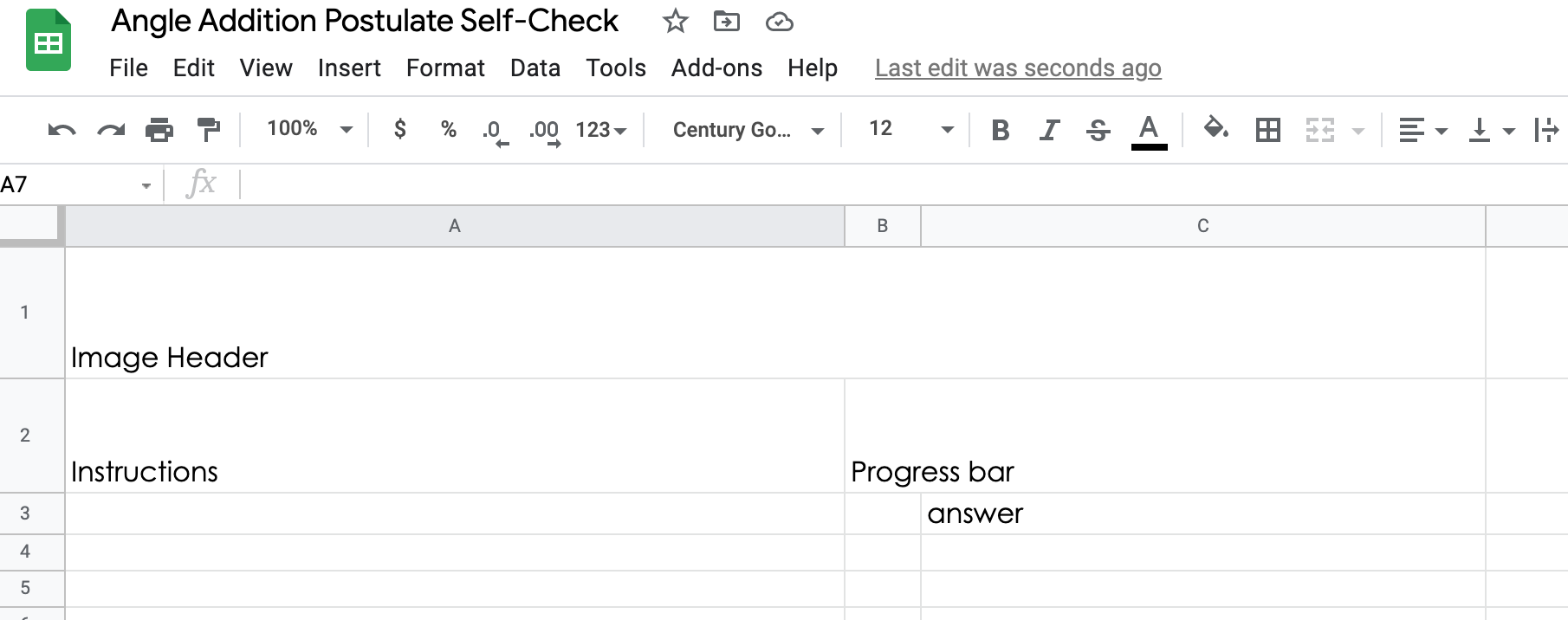
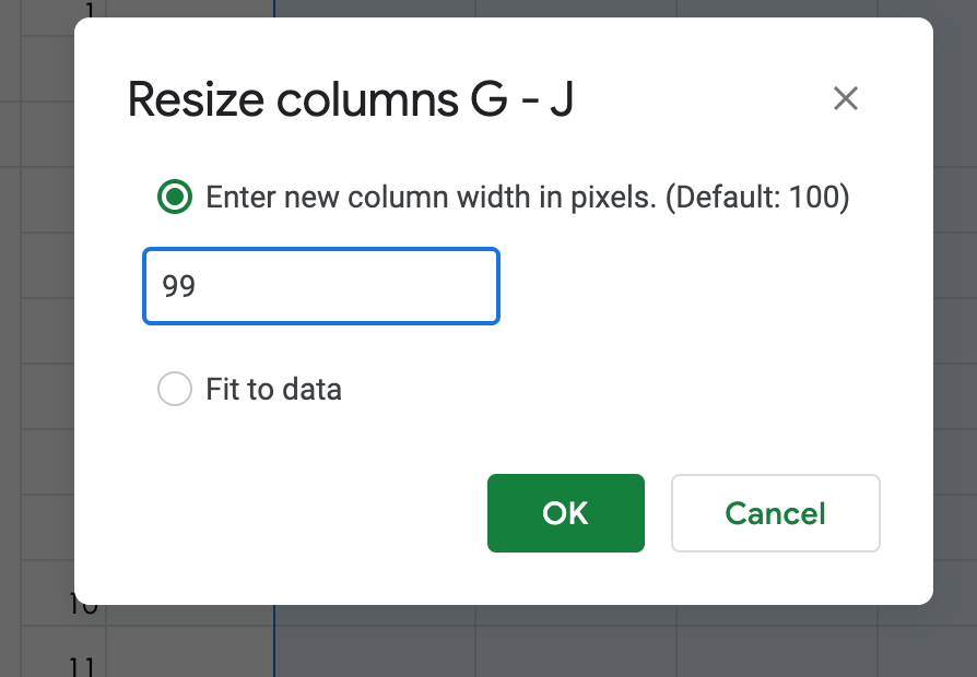
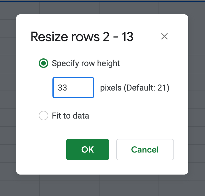
I start with my blocks of information. I merged cells to create the sections for instructions, question images, and also to create my grid. By selecting columns G-J and right clicking, I can resize my columns to 99. Do the same for rows 2-3 and resize to 33. This should give us squares.
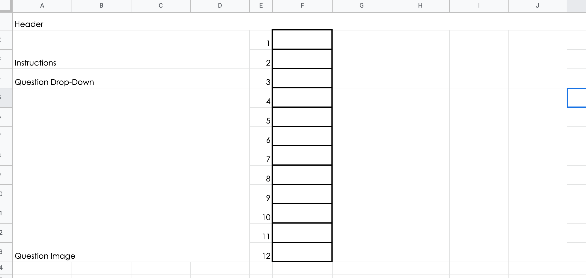
I just typed in my header this time, but you could always create a colorful header like we did the last time. If you create the header image, insert instructions are below.


Place images and answer in a new tab.
Click the plus button in the bottom left corner of your spreadsheet. This will create a new tab in Sheets. This will be the location for out images and answers.

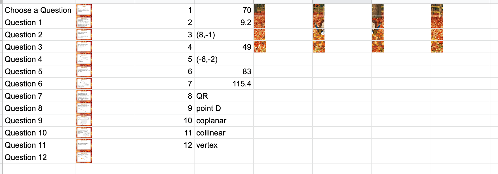
Place the images (insert image) for the questions and for the square reveal. They can be VERY TINY. It’s ok. It will scale to fit the size we allow it.
We also want to place the answers to our questions here. We are going to hide the tab later so students don’t see it.

Dropdown menu
Start with the dropdown menu where you have the word instructions. Place the same words, Choose a Question, Question 1, etc. in your list. You can view a tutorial here.
Now right below that, you will enter a vlookup code.
=vlookup(A4,Sheet2!A1:B13,2,0)
This is telling sheets to see what word is selected in A4 (Choose a question, Question 1, etc., then go to sheet 2 and select the image that matches my words that are in column A starting at A1 and my images are in column B ending at B13.
Answers
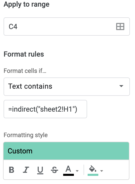
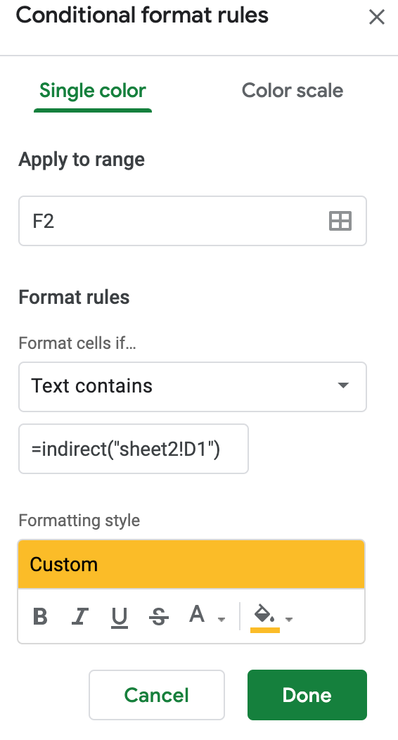
Now let’s set the conditional formatting for our answers. There is a tutorial for conditional formatting in the link above as well.
I’m going to have three rules for each cell. If the cell is empty, I want it to be transparent. If the cell has an entry it will be gold for correct or red for incorrect.
It’s a little tricky to get conditional formatting from another sheet.
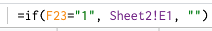
Here is what you would type in:
We will do the same thing to get a wrong answer but select text does not contain and type in the same formula and change the color to red.
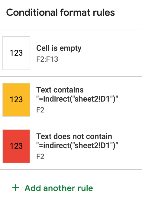
Repeat for the remaining answers.
*This seems like a lot of work, but this process allows you to use this template again simply by changing the images and answers in Sheet 2.
Load Image
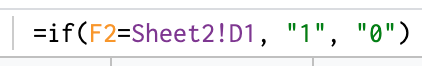
Now we need to load an image square. When an answer is correct, we want a square to load in an image space.
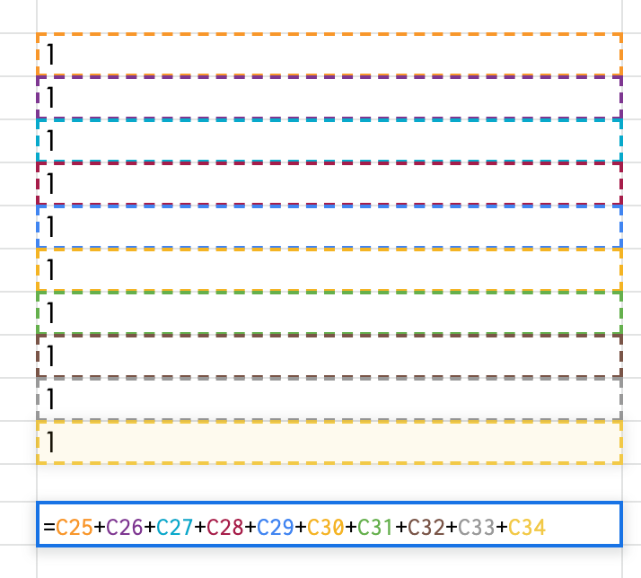
Below the fun stuff in Sheet 1, I have the sheet respond with 1 if an answer is correct and 0 if it’s incorrect using the following formula:
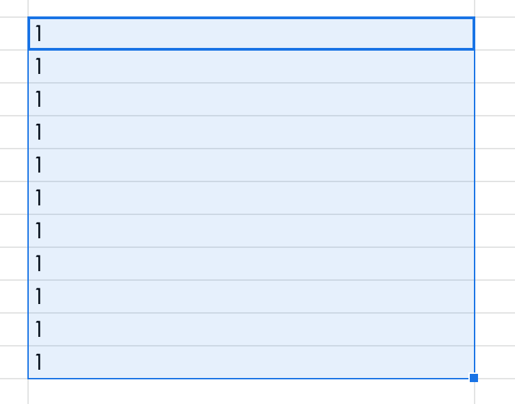
Once you return, there will be a little blue box in bottom right corner. You can drag that box down 10 spaces and it will auto fill the formula for you.
Choose a square you want to load. For this example, if the answer is correct it will go to sheet 2 and load the image in D1. You just need to make sure you load them in random order and that you include each one.
I have 16 boxes and only 12 questions so a few of my questions load to squares.

Clean it up and Assign
I like to hide the parts of the sheet we don’t need.
I’m going to highlight columns K-Z and right click and hide those cells

You can also hide the rows that have your adding trick on them by doing the same thing.
I’m also going to hide the sheet with my answers on it. Now a spreadsheet savvy student will now how to unhide this so you can always password protect the sheet so they can’t access it.

Don’t forget to set it to make a copy for every student in your LMS.
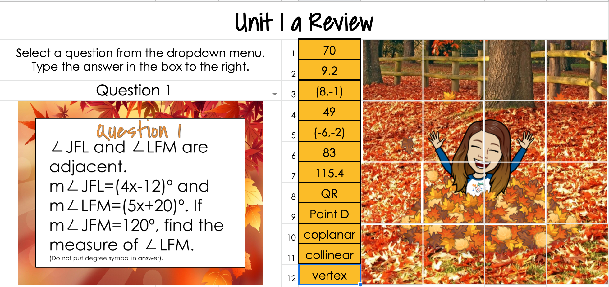
Here is the final result with all of the answers filled in:
These are so much fun. You can even get more advanced and have one image load and it changes to another image as you get the answer correct.
You can always just use the created spreadsheet below as a template if you don’t want to make your own. Just switch out the images and answers on Sheet 2.
If you make one, please let me know. I love to make these and my students love to complete these.