

It’s been a minute since we had a fun with Google Sheets so I decided to bring you another installment as school is starting or getting ready start for most of us.
Separate Names
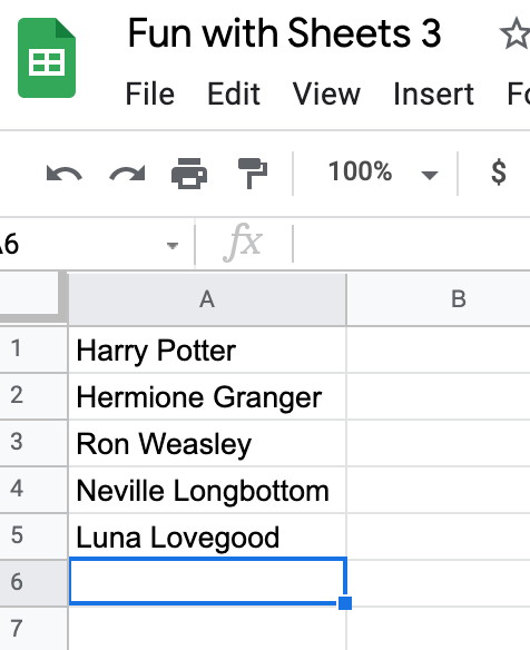
I like to copy the names of my students from my gradebook screen or download an Excel file of students from our grade management system (we use PowerSchool). This copies first and last names but sometimes I just need first names. I DON’T want to go through a delete all of the names, especially since I usually have around 150 students.
Never fear, Google Sheets are here! You can EASILY separate the names into two columns.
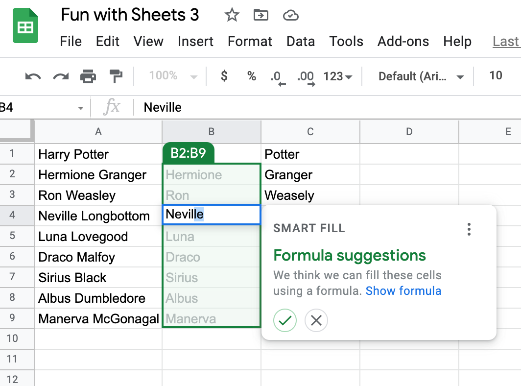
Begin by typing the names into two columns, just as you want them to appear. It may take a few names, but once Google Sheets understands what you are doing, Smart Fill will pop up a suggestion. Click the checkmark and Sheets will do the rest.
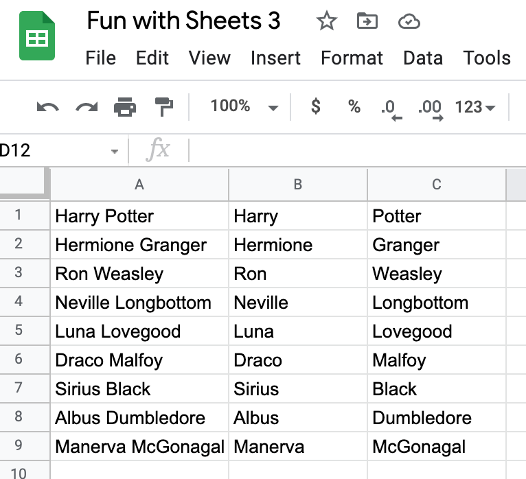
You will do the same for the last name column. Then you have the entire sheet broken into first and last names. YAY! Such a time saver.
The process also works in reverse. So if you have first and last names in two columns, you can type both in the third column and smart fill will recognize the pattern and fill for you.
Google Translate
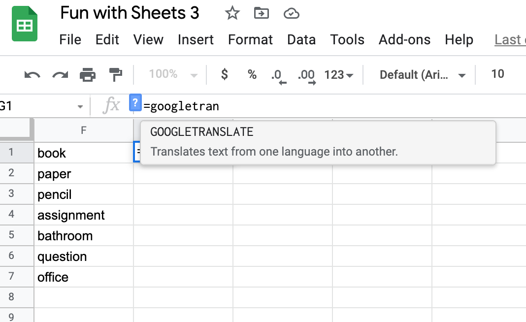
You can translate a list of words in Google Sheets. Type the list of words in one column. In the next column, type =googletranslate and and prompt will appear.
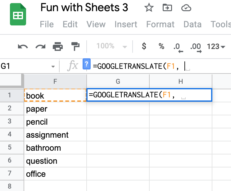
Next you want to click on the cell for the word you want to translate. Don’t worry, we don’t have to do this for every word, it will fill all of them in the end. It will place this cell into the formula, then put a comma and “auto” then a comma.
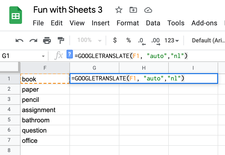
Now you need to find your two letter language code. These are called ISO codes and you can do a google search for them. Here is a link to the site I use. I’m translating to Dutch which is the code nl. So I will add the code in quotations and then close the parentheses.
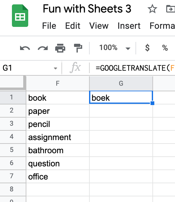
One word is translated.
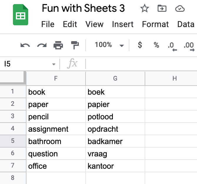
Now grab the blue box in the bottom right corner of that cell and drag down. You have translated all of the words.
Hiding Answers
I love to create interactive Google Slides for review games and escape room tasks. Most of the time the game works as it should. But every now and then a student figures out that you can click on the input box to see the answer. And, OF COURSE, they tell the rest of the class and now they are just entering the answer and not working out the problems.
Here is an example of a pixel art activity where this could be used. Many of mine have not been updated to this cell reference method but I will be updating them as I use them this year.
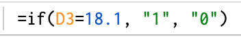
In this example, the student can see that typing 18.1 into D3 will give them the correct answer.
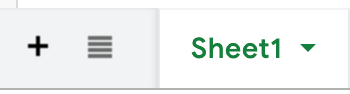
You can make this process more difficult for them. Using sheet 2 (click the + sign next to sheet 1 in the bottom row), you can type the answers into cells and then reference these cells on sheet 1.
I started in T33 to type my answers so it wasn’t on the screen if students click Sheet 2. You can also hide this sheet or password protect it so students can’t see it. If you do that, then just begin in A1 with your answers.
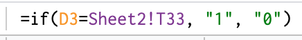
Replace 18.1 with Sheet2! followed by the cell where the answer is located, T33 for this example.
Now when a student clicks on the answers, they would have to unhide (if it’s not password protected) Sheet 2 then find T33 for the answer. I don’t usually password protect and it still deters most students.
Well, I hope you enjoyed this episode of Fun with Google Sheets and I hope you have a great start to your year!

1 thought on “Fun with Google Sheets – Part 3”