Self-Checking Google Sheets

Create your Questions

I find it’s easier to have my questions and images (if needed) ready to go before I begin building the spreadsheet.

I’m using this for Angle Addition Postulate so I’ve created my images in advance in a Google Slide and I changed the page size to the standard 4:3. I can download each card as a PNG or JPG image to use in my self-checking activity.

Progress Bar

For this type of self-checking activity you can have a progress bar or progress circle to tell students how many they have correct. Or you can just have the number of correct answers in the corner. For this tutorial, I’m going to use the progress bar

I drew my own, just for fun, but you could create these in Google Drawing or Google Slides. You will need one image for each increase in the bar or circle.

Open Sheets

Now we will put this all together.

I start with my blocks of information.

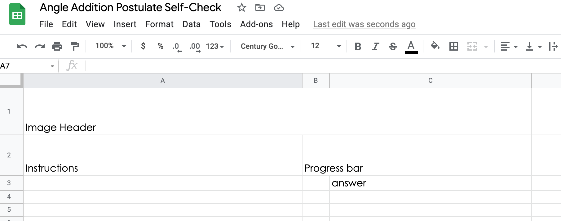
I created my header in Google Drawing. I will insert the image in the cell.

Place images and answer in a new tab.

Click the plus button in the bottom left corner of your spreadsheet. This will create a new tab in Sheets. This will be the location for out images and answers.

Place the images (insert image) for the questions and for the progress bar. They can be VERY TINY. It’s ok. It will scale to fit the size we allow it.

We also want to place the answers to our questions here. We are going to hide the tab later so students don’t see it.

Dropdown menu

Start with the dropdown menu where you have the word instructions. Place the same words, Choose a Question, Question 1, etc. in your list. You can view a tutorial here.

Now right below that, you will enter a vlookup code.

=vlookup(A3,Sheet2!D1:E12,2,0)

This is telling sheets to see what word is selected in A2 (Choose a question, Question 1, etc., then go to sheet 2 and select the image that matches my words that are in column D starting at D1 and my images are in column E ending at E12.

Answers

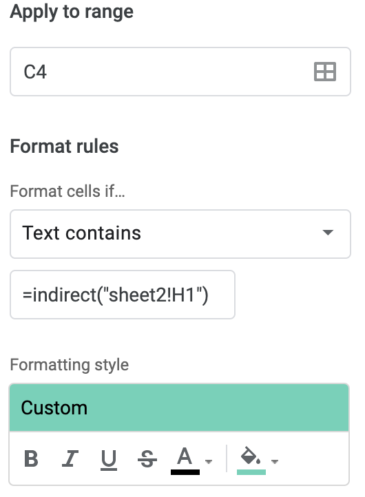
Now let’s set the conditional formatting for our answers. There is a tutorial for conditional formatting in the link above as well.

I’m going to have three rules for each cell. If the cell is empty, I want it to be transparent. If the cell has an entry it will be green for correct or yellow for incorrect.

It’s a little tricky to get conditional formatting from another sheet.

Here is what you would type in:

We will do the same thing to get a wrong answer but select text does not contain and type in the same formula and change the color to yellow.

Repeat for the remaining answers.

*This seems like a lot of work, but this process allows you to use this template again simply by changing the images and answers in Sheet 2.

Progress Bar

Now we need to add the progress bar. When an answer turns green, we want the progress bar to advance. Basically, you are adding the amount of correct answers together and telling the progress bar to load an image based on the number of correct answers.

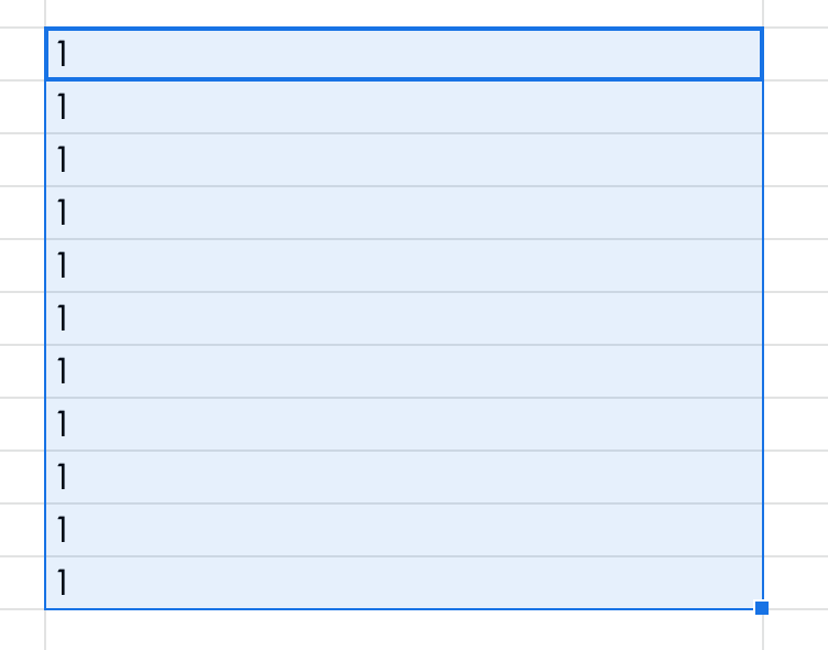
I have the number of correct answers add somewhere hidden on sheet 1 (below or to the right of the current content) using the following formula:

Once you return, there will be a little blue box in bottom right corner. You can drag that box down 10 spaces and it will auto fill the formula for you.

Now we will add the columns. We will use this sum to load the correct images. I will hide these rows (or columns) later so students don’t see it.

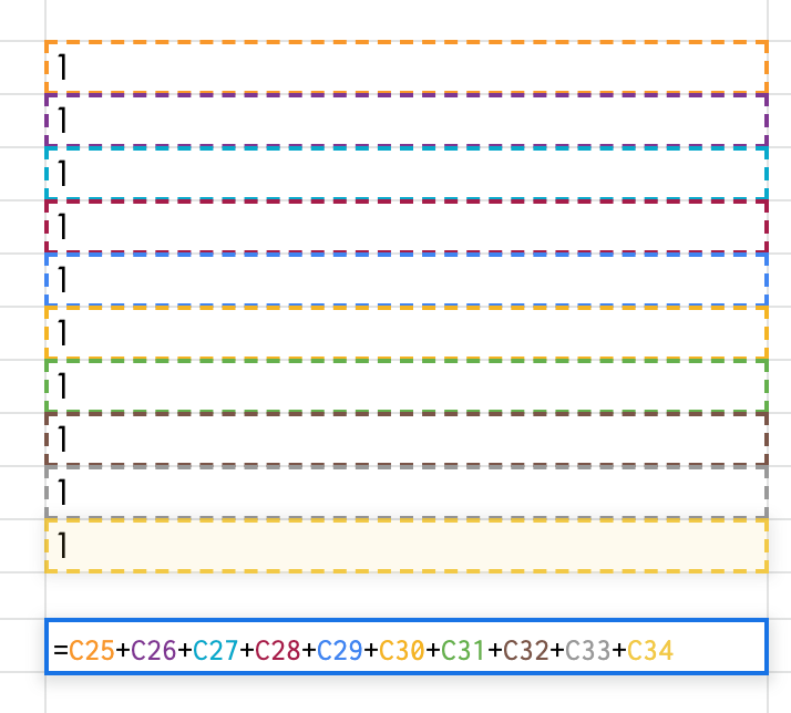
Usually the =sum feature will work but for some reason it didn’t, so I just added each cell.

In the cell where the progress bar goes, we are going to use that same vlookup that we used earlier to load the correct image:

Clean it up and Assign

I like to hide the parts of the sheet we don’t need.

I’m going to highlight D=Z and right click and hide those cells

You can also hide the rows that have your adding trick on them by doing the same thing.

I’m also going to hide the sheet with my answers on it. Now a spreadsheet savvy student will now how to unhide this so you can always password protect the sheet so they can’t access it.

Don’t forget to set it to make a copy for every student in your LMS.